Board Games
This is my first time participating in Tidy Tuesday AND my first blog post. My love for board games finally convinced me to actually post something to my blog.
In this post, I explore board game data from Board Game Geek and dive deeper into game mechanics to identify game mechanics that frequently co-occur in games.
I first loaded packages I knew I would be using as well as the data from the Tidy Tuesday GitHub.
library("tidyverse")
library("magrittr")
pal <- wesanderson::wes_palette("FantasticFox1", type = "discrete") # set color palette

board_games <- readr::read_csv("https://raw.githubusercontent.com/rfordatascience/tidytuesday/master/data/2019/2019-03-12/board_games.csv")
I wanted to first get a sense of board game ratings over time, contextualizing it by labeling some of my favorite games.
favorites <- c("Small World", "7 Wonders", "Dominion", "Codenames",
               "Betrayal at House on the Hill", "Citadels")

board_games %>%
  ggplot(aes(x = year_published, y = average_rating)) +
  geom_point(alpha = .25, color = pal[3]) +
  geom_smooth(method = "loess", span = .5, color = pal[5]) +
  ggrepel::geom_text_repel(data = . %>% filter(name %in% favorites),
            aes(label = name),size = 4.3) +
  geom_point(data = . %>% filter(name %in% favorites),
             aes(x = year_published, y = average_rating), size = 2) +
  labs(x = "Year published",
       y = "Average rating",
       title = "Average board game ratings increasing over time") +
  bbplot::bbc_style() +
  theme(axis.text=element_text(size=12),
        axis.title=element_text(size=14,face="bold"),
        plot.title=element_text(size=16,face="bold"))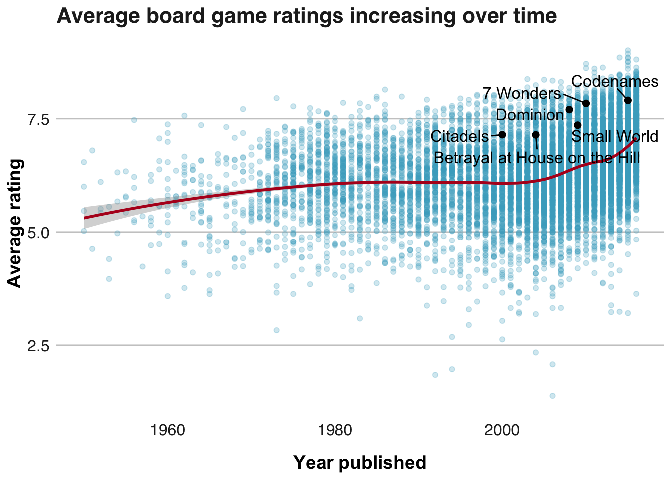
Figuring out how to selectively label and color only some data points was a useful exercise, and I rarely think to perform additional data manipulation inside a ggplot geom. Because the labeled points were so close together, the labels overlapped, making them hard to read. Luckily, the ggrepel package came to the rescue in spacing them out a bit more. They’re still a bit cramped, but much better than without it.
I’m also trying out the bbplot::bbc_style plot theme for all the graphs in this post, and I’m liking how clean the plots look.
Two takeaways from this graph:
- As noted by the FiveThirtyEight article that prompted the use of this data for Tidy Tuesday, board game ratings are increasing over time.
- I seem to have pretty good taste in board games, at least based on their average ratings :)
I also wanted to get a sense for how number of ratings and average ratings are related. Do more frequently rated games have higher average ratings?
board_games %>%
  ggplot(aes(x = users_rated, y = average_rating)) +
  geom_point(alpha = .25, color = pal[3]) +
  geom_smooth(method = "loess", span = .5) +
  scale_x_log10() +
  ggrepel::geom_text_repel(data = . %>% filter(name %in% favorites),
            aes(label = name),size = 4.3) +
  geom_point(data = . %>% filter(name %in% favorites),
             aes(x = users_rated, y = average_rating), size = 2) +
  labs(x = "Number of ratings (log)",
       y = "Average rating",
       title = "Average ratings increase with number of ratings") +
  bbplot::bbc_style() +
  theme(axis.text=element_text(size=12),
        axis.title=element_text(size=14,face="bold"),
        plot.title=element_text(size=16,face="bold"))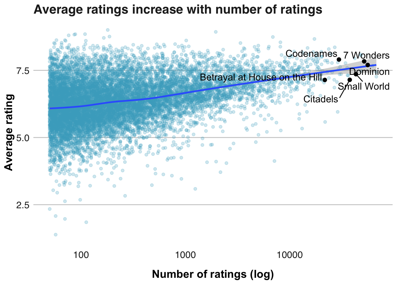
It does seem that more frequently rated games also have higher ratings, and all of my favorite games are also have a lot of ratings.
Game Characteristics
What do the other game attributes look like? Specifically I was interested in a game’s expansions and mechanics, which were each stored in a single column, with multiple expansions and mechanics separated by commas. I used splitstackshape::concat.split to create list columns inside the tibble with those values, then counted the number of items in the list for each game to get a count of expansions and mechanics. Minimum number of players also had a long tail, with values above 5 infrequent, so I lumped those into one category.
board_games <- board_games %>%
  splitstackshape::concat.split("expansion", sep = ",", structure = "list") %>%
  splitstackshape::concat.split("mechanic", sep = ",", structure = "list") %>%
  mutate(expansion_n = map_dbl(expansion_list, function(x) sum(!is.na(x))),
        mechanic_n = map_dbl(mechanic_list, function(x) sum(!is.na(x)))) %>%
  mutate(min_players_fct = as.factor(case_when(min_players == 0 ~ NA_character_,
                                                  min_players == 1 ~ "1",
                                                  min_players == 2 ~ "2",
                                                  min_players == 3 ~ "3",
                                                  min_players == 4 ~ "4",
                                                  min_players >= 5 ~ "5+",
                                                  TRUE ~ NA_character_)))
p1 <- ggplot(board_games, aes(x = min_players_fct)) +
geom_bar(fill = pal[1], stat = "count") +
labs(x = "Minimum number of players",
y = "Number of games") +
bbplot::bbc_style() +
theme(axis.text=element_text(size=10),
axis.title=element_text(size=12,face="bold"))
p2 <- filter(board_games, playing_time <= 600) %>%
ggplot(aes(x = playing_time)) +
geom_histogram(fill = pal[1], bins = 15) +
labs(x = "Play time (min.)",
y = "Number of games") +
bbplot::bbc_style() +
theme(axis.text=element_text(size=10),
axis.title=element_text(size=12,face="bold"))
p3 <- ggplot(board_games, aes(x = mechanic_n)) +
geom_histogram(fill = pal[1], bins = 20) +
labs(x = "Number of mechanics",
y = "Number of games") +
bbplot::bbc_style() +
theme(axis.text=element_text(size=10),
axis.title=element_text(size=12,face="bold"))
p4 <- filter(board_games, expansion_n < 100) %>%
ggplot(aes(x = expansion_n)) +
geom_histogram(fill = pal[1], bins = 50) +
labs(x = "Number of expansions",
y = "Number of games") +
bbplot::bbc_style() +
theme(axis.text=element_text(size=10),
axis.title=element_text(size=12,face="bold"))
p <- cowplot::plot_grid(p1, p2, p3, p4, nrow = 2)
title <- cowplot::ggdraw() +
cowplot::draw_label("Distributions of game characteristics",
fontface='bold', size = 16)
cowplot::plot_grid(title, p, ncol = 1, rel_heights=c(0.1, 1))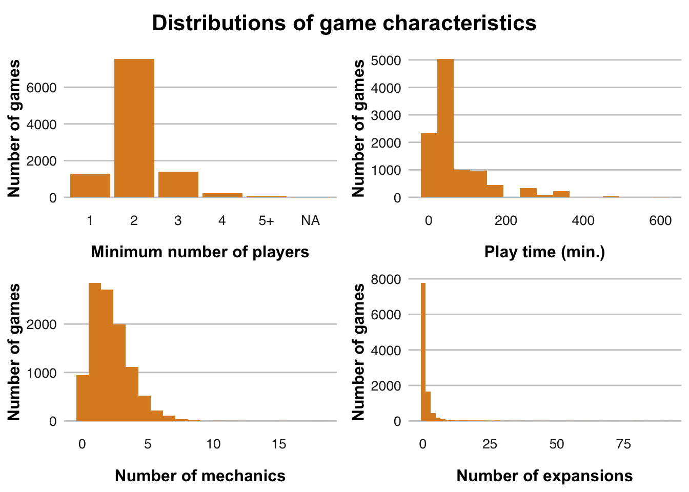
The cowplot package helped me get all four plots into one figure. Most games require a minimum of two players, and the median play time is 45 minutes. The plot only shows games <=10 hours, but there were 56 board games with play time over 10 hours. These are likely a mix of games played over multiple sessions and erroneous data.
Most games employ several game mechanics, and most games don’t have any expansions, but there were 9 games with more than 100 expansions that I removed from the plot, including one game with 420 expansions!
Game Mechanics
I was most interested in further exploring the game mechanics, and since each game can have multiple mechanics, I used tidyr::separate_rows to get each mechanic on its own line.
board_games_mech <- board_games %>%
  tidyr::separate_rows(mechanic, sep = ",") %>%
  filter(!is.na(mechanic)) %>%
  group_by(mechanic) %>%
  add_tally() %>%
  ungroup() %>%
  mutate(mechanic = fct_reorder(mechanic, n))

p5 <- board_games_mech %>%
  ggplot(aes(x = mechanic)) +
  geom_bar(stat = "count", fill = pal[5]) +
  coord_flip() +
  labs(x = "Game mechanic",
      y = "Number of games") +
  bbplot::bbc_style() +
  theme(axis.text=element_text(size=8),
        axis.title=element_text(size=12,face="bold"))

p6 <- board_games_mech %>%
  ggplot(aes(x = mechanic, y = average_rating)) +
  geom_boxplot() +
  coord_flip() +
    theme(axis.text.y = element_blank(),
        axis.title.y = element_blank()) +
  labs(y = "Average rating") +
  bbplot::bbc_style() +
  theme(axis.text=element_text(size=8),
        axis.title=element_text(size=12,face="bold"))

pp <- cowplot::plot_grid(p5, p6, nrow = 1)
title <- cowplot::ggdraw() + cowplot::draw_label("Number of ratings and average rating of games by mechanic", fontface='bold', size = 16)
cowplot::plot_grid(title, pp, ncol = 1, rel_heights=c(0.1, 1))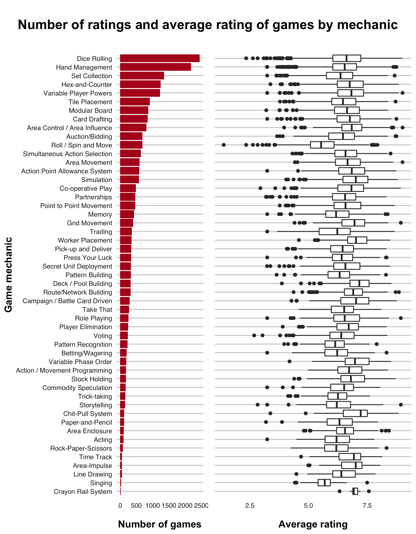
board_games_mech %>%
  group_by(mechanic) %>%
  summarize(n = n(), average_rating = mean(average_rating)) %>%
  ggplot(aes(x = n, y = average_rating)) +
  geom_point(color = pal[5]) +
    labs(x = "Number of games",
       y = "Average rating",
       title = "Number of games and average rating of games by mechanic") +
  bbplot::bbc_style() +
  theme(axis.text=element_text(size=8),
        axis.title=element_text(size=12,face="bold"),
        plot.title=element_text(size=16,face="bold"))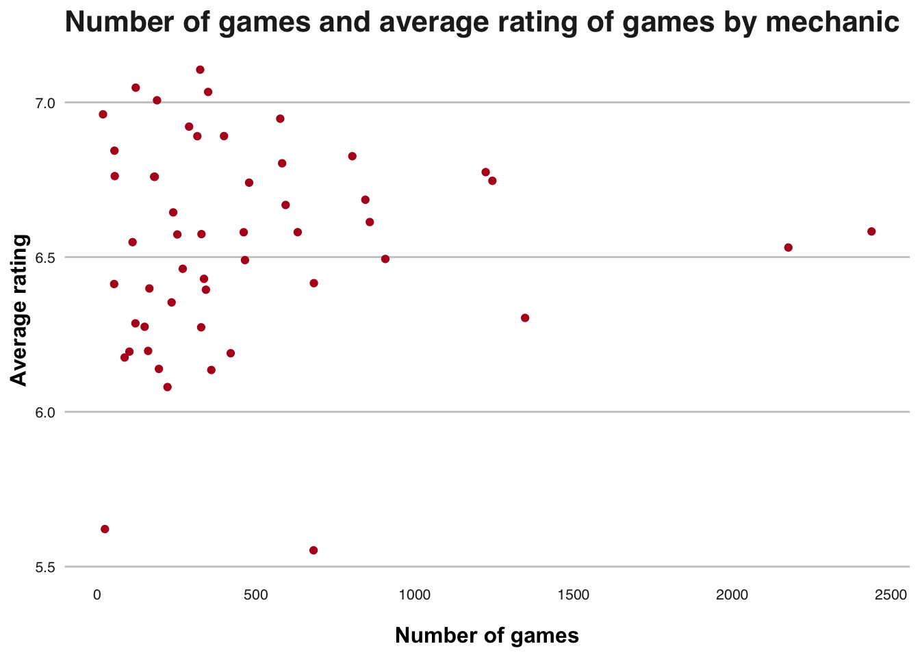
There are 51 different mechanics, with Dice Rolling and Hand Management being the most frequent. There is some variability in rating across mechanics, and the ratings of the games in a mechanic do not seem related to the number of games in that mechanic. Notably, Roll/Spin and Move stands out as having comparably lower ratings.
I’m not familiar with what all of these mechanics actually mean, so I wanted to see the highest rated and most rated game in the most popular mechanics to get an idea of the type of games that use those mechanics.
board_games_mech %>%
  group_by(mechanic) %>%
  summarize(top_rated = first(name, order_by = desc(average_rating)), most_rated = first(name, order_by = desc(users_rated))) %>%
  arrange(desc(mechanic)) %>%
  head(10) %>%
kable()| mechanic | top_rated | most_rated |
|---|---|---|
| Dice Rolling | Small World Designer Edition | Catan |
| Hand Management | Through the Ages: A New Story of Civilization | Catan |
| Set Collection | Pandemic Legacy: Season 1 | Pandemic |
| Hex-and-Counter | Last Chance for Victory | Twilight Imperium (Third Edition) |
| Variable Player Powers | Small World Designer Edition | Pandemic |
| Tile Placement | 1817 | Carcassonne |
| Modular Board | Mechs vs. Minions | Catan |
| Card Drafting | Through the Ages: A New Story of Civilization | Dominion |
| Area Control / Area Influence | Small World Designer Edition | Carcassonne |
| Auction/Bidding | Through the Ages: A New Story of Civilization | Power Grid |
Board Game Mechanic Association Rules
Since games frequently have multiple mechanics, are there game mechanics that commonly co-occur? To answer this question, I used association rules to identify commonly co-occurring game mechanics. In order to use the arules package for association rule mining, the data has to be in “transactions” format. In order to get it in this format, I first restructured the data so that each mechanic was on its own line. From there, I transformed the data into a list, where each item in the list represents a single game and contains a factor array of that game’s mechanic(s). This can then be converted into “transactions” format.
library("arules")
library("arulesViz")

board_games_mech <- board_games %>%
  select(game_id, mechanic) %>%
  tidyr::separate_rows(mechanic, sep = ",") %>%
  filter(!is.na(mechanic)) %>%
  group_by(game_id) %>%
  # filter(n() > 1) %>% # removing games with only one mechanic
  ungroup() %>%
  mutate_all(as.factor)

mechanics_list <-  split(board_games_mech$mechanic, board_games_mech$game_id)
mechanics_transactions <- as(mechanics_list, "transactions")
summary(mechanics_transactions)
> transactions as itemMatrix in sparse format with
> 9582 rows (elements/itemsets/transactions) and
> 51 columns (items) and a density of 0.04900938
>
> most frequent items:
> Dice Rolling Hand Management Set Collection
> 2438 2176 1347
> Hex-and-Counter Variable Player Powers (Other)
> 1244 1223 15522
>
> element (itemset/transaction) length distribution:
> sizes
> 1 2 3 4 5 6 7 8 9 10 11 12 15 18
> 2852 2716 1987 1113 524 217 111 30 23 4 2 1 1 1
>
> Min. 1st Qu. Median Mean 3rd Qu. Max.
> 1.000 1.000 2.000 2.499 3.000 18.000
>
> includes extended item information - examples:
> labels
> 1 Acting
> 2 Action / Movement Programming
> 3 Action Point Allowance System
>
> includes extended transaction information - examples:
> transactionID
> 1 1
> 2 2
> 3 3The board game data is now stored as a matrix. The density in a sparse matrix indicates the proportion of non-empty cells: 0.05. The most frequent items and itemset/transaction length distribution match the distributions above, showing that Dice Rolling is the most frequent mechanic, and 2852 games only have one mechanic. If I had not already done this exploratory analysis, I would usually use itemFrequencyPlot to visualize the most frequent mechanics.
First, I’m using the frequent itemsets target to find combinations of game mechanics that commonly occur together.
itemsets <- apriori(mechanics_transactions,
                    parameter = list(supp=0.01, minlen = 2, maxlen=5,
target = "frequent itemsets"))summary(itemsets)> set of 73 itemsets
>
> most frequent items:
> Dice Rolling Hand Management
> 26 19
> Variable Player Powers Set Collection
> 16 10
> Area Control / Area Influence (Other)
> 9 72
>
> element (itemset/transaction) length distribution:sizes
> 2 3
> 67 6
>
> Min. 1st Qu. Median Mean 3rd Qu. Max.
> 2.000 2.000 2.000 2.082 2.000 3.000
>
> summary of quality measures:
> support count
> Min. :0.01012 Min. : 97.0
> 1st Qu.:0.01158 1st Qu.:111.0
> Median :0.01472 Median :141.0
> Mean :0.01810 Mean :173.5
> 3rd Qu.:0.01993 3rd Qu.:191.0
> Max. :0.05469 Max. :524.0
>
> includes transaction ID lists: FALSE
>
> mining info:
> data ntransactions support confidence
> mechanics_transactions 9582 0.01 1There are 73 combinations of mechanics that occur in at least 1% of the data: 67 two mechanic combinations, and 6 three mechanic combinations.
One important metric for frequent itemsets is support, which indicates how frequently the itemset appears in the data set, or the proportion of games that contain the combination of mechanics.
Below are the 10 mechanic combinations with the highest support. The most frequent combination of mechanics is Dice Rolling and Variable Player Powers, which occurred in about 5.5% of all games. This combination makes sense, because those two mechanics occurred with high frequency (they were the 1st and 4th highest, respectively). Interestingly, the combination of the two most frequent mechanics, Dice Rolling and Hand Management, only occurs 6th most frequently as a pair.
DATAFRAME(itemsets) %>%
  arrange(desc(support)) %>%
  head(10) %>%
  rename("mechanics" = items) %>%
kable(row.names = F, digits = 3)| mechanics | support | count |
|---|---|---|
| {Dice Rolling,Variable Player Powers} | 0.055 | 524 |
| {Hand Management,Set Collection} | 0.045 | 430 |
| {Dice Rolling,Hex-and-Counter} | 0.044 | 420 |
| {Hand Management,Variable Player Powers} | 0.041 | 392 |
| {Card Drafting,Hand Management} | 0.039 | 374 |
| {Dice Rolling,Hand Management} | 0.036 | 344 |
| {Dice Rolling,Modular Board} | 0.034 | 322 |
| {Hex-and-Counter,Simulation} | 0.031 | 295 |
| {Area Movement,Dice Rolling} | 0.028 | 268 |
| {Dice Rolling,Simulation} | 0.028 | 265 |
Moving on to association rule mining, which gives output in the form of if this then that rules. For example, if a game employs mechanic X, it is likely to also employ mechanic Y.
association_rules <- apriori(mechanics_transactions,
parameter = list(supp=0.001, conf=0.8, maxlen=5))summary(association_rules)> set of 51 rules
>
> rule length distribution (lhs + rhs):sizes
> 3 4 5
> 9 37 5
>
> Min. 1st Qu. Median Mean 3rd Qu. Max.
> 3.000 4.000 4.000 3.922 4.000 5.000
>
> summary of quality measures:
> support confidence lift count
> Min. :0.001044 Min. :0.8000 Min. : 3.144 Min. :10.00
> 1st Qu.:0.001148 1st Qu.:0.8363 1st Qu.: 3.983 1st Qu.:11.00
> Median :0.001357 Median :0.8667 Median : 7.123 Median :13.00
> Mean :0.002089 Mean :0.8826 Mean :10.141 Mean :20.02
> 3rd Qu.:0.001513 3rd Qu.:0.9253 3rd Qu.:11.109 3rd Qu.:14.50
> Max. :0.007201 Max. :1.0000 Max. :30.419 Max. :69.00
>
> mining info:
> data ntransactions support confidence
> mechanics_transactions 9582 0.001 0.8There are 51 association rules that occur in at least .1% of the data. The support threshold is very low for association rules because there are so many games with only one mechanic that don’t fit any association rules.
Association rule mining employs an additional metric, confidence, which indicates how often the rule is true, or the proportion of games that have the left hand side (LHS) that also contain the right hand side (RHS). Crayon Rail System only appears in <1% of games, but 86% of the time a game is labeled as both Crayon Rail System and Route/Network Building, it is also labeled as Pick-up and Deliver, with this association rule occurring in 12 games.
DATAFRAME(association_rules) %>%
  head(11) %>%
kable(row.names = F, digits = 3)| LHS | RHS | support | confidence | lift | count |
|---|---|---|---|---|---|
| {Crayon Rail System,Route/Network Building} | {Pick-up and Deliver} | 0.001 | 0.857 | 24.015 | 12 |
| {Crayon Rail System,Pick-up and Deliver} | {Route/Network Building} | 0.001 | 0.857 | 26.073 | 12 |
| {Stock Holding,Tile Placement} | {Route/Network Building} | 0.005 | 0.839 | 25.530 | 47 |
| {Deck / Pool Building,Take That} | {Hand Management} | 0.001 | 0.824 | 3.626 | 14 |
| {Partnerships,Role Playing} | {Variable Player Powers} | 0.004 | 0.800 | 6.268 | 40 |
| {Role Playing,Tile Placement} | {Modular Board} | 0.001 | 0.857 | 9.572 | 12 |
| {Route/Network Building,Trading} | {Dice Rolling} | 0.001 | 0.875 | 3.439 | 14 |
| {Auction/Bidding,Roll / Spin and Move} | {Trading} | 0.007 | 0.862 | 23.021 | 69 |
| {Auction/Bidding,Roll / Spin and Move} | {Set Collection} | 0.007 | 0.850 | 6.047 | 68 |
| {Auction/Bidding,Stock Holding,Tile Placement} | {Route/Network Building} | 0.002 | 1.000 | 30.419 | 23 |
| {Auction/Bidding,Roll / Spin and Move,Stock Holding} | {Trading} | 0.001 | 1.000 | 26.691 | 11 |
Below are the 10 association rules with the highest confidence. For the first 5, in 100% of the games that the combination of LHS mechanics occur, the RHS mechanic occurs as well. So 100% of the games labeled as Auction/Bidding, Stock Holding, and Tile Placement are also labeled as Route/Network Building, and this association occurs in 23 games.
DATAFRAME(association_rules) %>%
  arrange(desc(confidence)) %>%
  head(10) %>%
kable(row.names = F, digits = 3)| LHS | RHS | support | confidence | lift | count |
|---|---|---|---|---|---|
| {Auction/Bidding,Stock Holding,Tile Placement} | {Route/Network Building} | 0.002 | 1.000 | 30.419 | 23 |
| {Auction/Bidding,Roll / Spin and Move,Stock Holding} | {Trading} | 0.001 | 1.000 | 26.691 | 11 |
| {Roll / Spin and Move,Set Collection,Stock Holding} | {Trading} | 0.001 | 1.000 | 26.691 | 11 |
| {Grid Movement,Modular Board,Role Playing,Variable Player Powers} | {Dice Rolling} | 0.001 | 1.000 | 3.930 | 13 |
| {Area Control / Area Influence,Area Movement,Campaign / Battle Card Driven} | {Dice Rolling} | 0.002 | 0.952 | 3.743 | 20 |
| {Auction/Bidding,Roll / Spin and Move,Set Collection} | {Trading} | 0.007 | 0.941 | 25.121 | 64 |
| {Grid Movement,Modular Board,Role Playing} | {Dice Rolling} | 0.002 | 0.938 | 3.685 | 15 |
| {Grid Movement,Role Playing,Variable Player Powers} | {Dice Rolling} | 0.001 | 0.933 | 3.668 | 14 |
| {Dice Rolling,Partnerships,Role Playing} | {Variable Player Powers} | 0.001 | 0.933 | 7.313 | 14 |
| {Co-operative Play,Dice Rolling,Point to Point Movement} | {Variable Player Powers} | 0.001 | 0.933 | 7.313 | 14 |
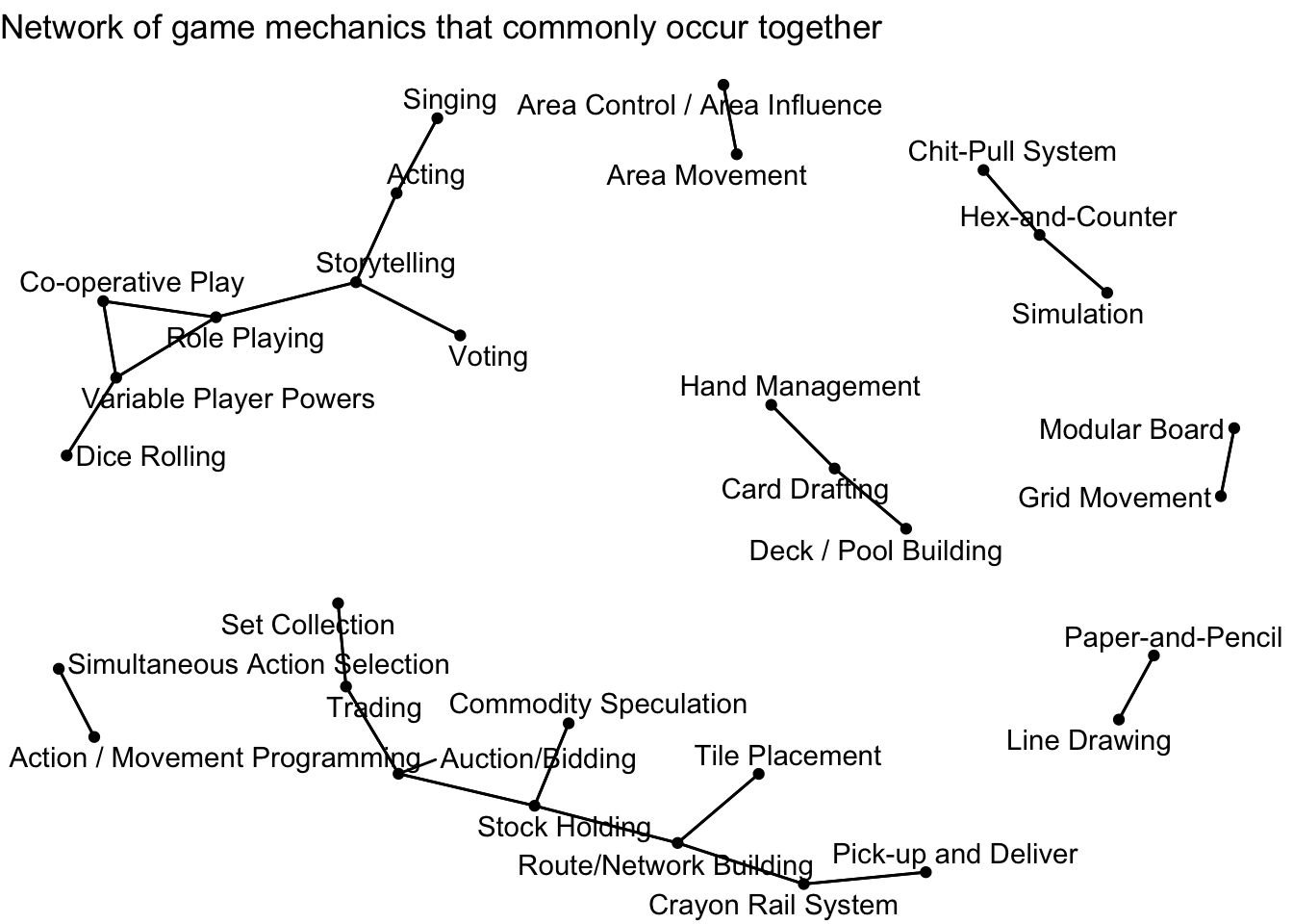
Network graph of game mechanics
This shows constellations of mechanics that frequently occur together.
require(widyr)
require(igraph)
require(ggraph)
require(ggforce)

board_games %>%
  select(name, mechanic) %>%
  tidyr::separate_rows(mechanic, sep = ",") %>%
  filter(!is.na(mechanic)) %>%
  mutate_all(as.factor) %>%
  pairwise_cor(mechanic, name, sort = T) %>%
  filter(correlation > .15) %>%
  graph_from_data_frame() %>%
  ggraph() +
  geom_edge_link() +
  geom_node_point() +
  geom_node_text(aes(label = name), repel = T) +
  theme_void() +
  labs(title = "Network of game mechanics that commonly occur together")